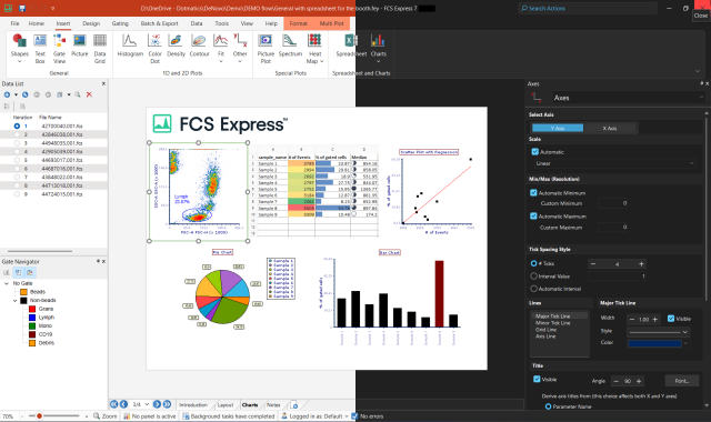
![]() ![]() ![]() |
![]() |
If you have any questions which do not appear on this list, please do not hesitate to contact us directly.
What is Biexponential and Hyperlog scaling?Biexponential and Hyperlog™ are equations that are characterized by exhibiting pseudo-linear like behaviour values near a reflection point (usually zero) and transitioning to pseudo-logarithmic behaviour at values distant from the reflection point. These equations are often used to display flow cytometry data with a high dynamic range (usually >16 bits) on a single plot. They are preferred to the logarithmic scale mainly for the following characteristics:
The following articles provide more detailed information than can be found in this web page: A general review on scaling displays in flow
cytometry: A detailed description of the Hyperlog transformation: A detailed description of the Biexponential transformation: The key adjustable parameter of these equations is the reflection point, i.e. at what point along the data does the equation transition from linear-like to log-like behaviour. Since the biexponetial display was popularized by the BD FACSDiva software, we will begin our discussion there. Biexponential and the BD FACSDiva SoftwareThe FACSDiva™ software allows you to view a parameter on a biexponential scale by opening the inspector for the plot (View->Inspector) and setting the checkbox for the the axis you wish to show as biexponential, as in the image below.![]() By default, the FACSDiva software calculates the reflection point automatically. FACSDiva uses a proprietary algorithm to calculate the reflection point (it is not the method suggested in the Parks et. al. paper above) in order to optimize the biexponential display for data generated by BD instruments. The FACSDiva software does not tell you what reflection point it calculated, but it does tell you a "below zero" value. This below zero value can be considerered to be approximately the lowest data value that will be plotted on your plot (this is not exactly correct, but is a close enough approximation). It is important to note that there may be data in your data file that is not actually plotted on the plot. This is particularly true if there are a few outlying events that are much more negative than the bulk of your population. The algorithm is designed to ignore these events, so that these few events do not unduly influence the entire plot. If they were not ignored, there could be a large amount of area on your graph devoted to just a few cells. Thus, it is important to reiterate that, by default, the below zero value can change from data file to data file. That means that even though two plots may look similar, one may have to closely inspect axes to see if the axes vary widely from plot to plot. Please see the paper by Novo & Wood above for a more detailed explanation and examples. It is possible to view the below zero value by opening the Biexponential Editor in the FACSDiva software (View->Biexponential Editor), as in the image below ![]() Note that the below zero value has been automatically calculated for each of the parameters in the data file. You can enter the Below Zero value yourself by selecting the Manual radio button and entering the values you desire. You would manually enter values if you wanted the axis scaling to be consistent from sample to sample. By default, the below zero is calculated based on all events, however FACSDiva also allows you to choose the population that it will use to automatically calculate the below zero value. You can select this by right clicking on a plot and selecting Scale to Population and then choosing the population you want, as in the image below:
You can see in the two images below that the scale-to population can have a dramatic effect. Setting the scale to population to a particular population will have the effect of trying to make the lowest cluster of data in that population appear as a cluster in the area of the plot immediately adjacent to the axis. In the left panel below, notice the minimum value on the Y-axis is -6,011. This is due to there being some events (red box ) that are much more negative than the rest of the population. Most of these events are not in the P1 population. By changing the scale-to to be based on P1 (right panel) the below zero calculation does not consider the events that are outside P1, which includes most of the events in the red box. Thus, the below zero value is much more positive (only -1,282) in the panel on the right.
Biexponential and Hyperlog Scaling with FCS ExpressAs a result of our close collaboration with BD, FCS Express now supports all of the options that FACSDiva does in terms of displaying biexponential data. In fact, we have implemented FACSDiva's proprietary algorithm for calculating the reflection point, so the results from FCS Express will look identical to the results from the FACSDiva software. FCS Express supports a wide variety of scaling formuli. To set the scaling on a plot, right click on the plot and select Format from the popup menu that appears. Then select the Axis category, as in the image below. You can set the scaling independently for each axis, and choose from a wide variety of scaling formuli. The different formuli are explained in detail in the FCS Express manual.
Each scaling formula also has different options associated with it. These options appear immediately below the scaling combo box when you select a particular scaling in FCS Express. ![]() The hyperlog scaling equation only has a single adjustable parameter, corresponding to the b variable in the Bagwell paper. This parameter can be thought of as the channel value below which the scaling exhibits predominantly linear like behaviour. The biexponential options are more complicated, and are shown in the image below. We will describe each property in detail.![]() The Current value on plot (red arrow above) shows the current below zero value that is being used on that plot. If you change any of the biexponential parameters and press Preview on the format screen, this value will update immediately to reflect the new below zero value that was calculated based on the new settings. When the automatic checkbox is set, as in the image above, the below zero value will be set based on the below zero value that was stored in the FCS file. When the automatic checkbox is checked, all of the specific biexponential options are disabled. In order to enable the different options, uncheck the automatic checkbox. ![]() When the automatic checkbox is unchecked, the plot will use the biexponential options from the format screen to set the below zero value, and not use the below zero value from the FCS file. If you select the Use this value radio button (image above, red arrow) then the plot will use the below zero value that you entered (in the image above, 200). Selecting a fixed below zero value is recommended if you wish the axis scaling on the plot to be consistent from sample to sample. If you wish to have the below zero value adjust automatically based on the data, you can select the Calculate automatically radio button (red arrow in the image below). This will mimic the default behaviour in FACSDiva. When you choose calculate automatically you will be give two additional choices.
When you open a plot in FCS Express with a FACSDiva data file, using FCS Express' default User Preferences, it will endeavour to display the data in the same way as you were looking at it in FACSDiva - in linear, log or biex, and using the same biex "below zero" values. In most cases, FCS Express will show the plot using the previously calculated value from FACSDiva. However, if you had chosen a Scale-To Population in FACSDiva, FCS Express will not be able to match the values, because they are not stored in the data file. In that case, you will be able to recreate the way it looked by using the formatting options described above. The figure below shows a comparison of the data from FACSDiva and FCS Express.
The FACSDiva ImporterThe BD FACSDiva importer in FCS Express will import your experiments from the FACSDiva software and recreate a similar analysis in FCS Express. More information can be found here. Prior to FCS Express version 3.00.0800, plots that were shown in biexponential in FACSDiva were imported as hyperlog in FCS Express. However, versions subsequent to 3.00.0800 will preserve the biexponential scaling when the experiments are imported into FCS Express. (To check your version number, go to Help->About from the main menu). Unfortunately, if you selected a Scale-To Population in FACSDiva, FCS Express will not be able to set up the "with the gate" option described above to be the same as the scale-to population. This is because the FACSDiva exported XML file does not contain the name of the scale-to population that was chosen. You will have to go to the plots in FCS Express and select the proper gate yourself. Hyperlog is a trademark of Verity Software
|
|||||||||||||
| Copyright © De Novo Software 2009. All rights reserved. Privacy Policy Terms of Use | ||||||||||||||